Today we are going to go back and learn a bunch of super useful data managmenet functions. In orer to do so, we are going to learn a bit of new language which is taken from SQL. If you’re serious about data, you’ll most likely want to learn to learn some SQL at some point. Let’s look at this great diagram here. You should always have a sense of the dimensions of any object that occurs as a result of the join.
There are three main ways of implementing joins in R. Base has merge, while plyr has join() and dplyr has a all of the various types like inner_join(). Let’s go fo a deep dive in to joins.
library(plyr)
library(dplyr)
library(reshape2)
set.seed(2015)
leftData <- data.frame(letters = LETTERS[1:5], sequence = seq(1,5), stringsAsFactors = FALSE) #LETTERS is a constant ?LETTERS
rightData <- data.frame(letters = LETTERS[1:5], rand = rnorm(5), stringsAsFactors = FALSE)
print(leftData)## letters sequence
## 1 A 1
## 2 B 2
## 3 C 3
## 4 D 4
## 5 E 5print(rightData)## letters rand
## 1 A -1.545448388
## 2 B -0.528393243
## 3 C -1.086758791
## 4 D -0.000111512
## 5 E 0.388953783This is the most simple situation. In fact, here we don’t even need an explicit join because the columns are all in the correct order. This is known as an implict join.
implictJoin <- cbind(leftData, rightData[, 2])Why is this a bad idea?
We want to enforce the matching on what is often known as a key. An implict join wouldn’t works if our data looked like this.
leftData <- leftData[sample(1:nrow(leftData)), ]
print(leftData)
## letters sequence
## 4 D 4
## 2 B 2
## 1 A 1
## 3 C 3
## 5 E 5We could sort the data, but generally we actually want to think about the type of the join. In this case we know the dimensions, and we know that they are the same, but often good to check.
nrow(leftData) == nrow(rightData)## [1] TRUEsetdiff(leftData$letters, rightData$letters)## character(0)intersect(leftData$letters, rightData$letters)## [1] "D" "B" "A" "C" "E"leftJoinM <- merge(leftData, rightData, by = "letters")
#finds all the names in come and joins. But ONLY key names have to be the same!
leftJoinJ <- join(leftData, rightData, type = "left") ## Joining by: lettersleftJoinIJ <- left_join(leftData, rightData)## Joining by: "letters"(leftJoinIJ == leftJoinJ) == leftJoinM # why## letters sequence rand
## [1,] FALSE TRUE FALSE
## [2,] FALSE FALSE FALSE
## [3,] FALSE FALSE FALSE
## [4,] FALSE FALSE FALSE
## [5,] FALSE FALSE FALSEprint(list(left_join = leftJoinIJ, join = leftJoinJ, merge = leftJoinM))## $left_join
## letters sequence rand
## 1 D 4 -0.000111512
## 2 B 2 -0.528393243
## 3 A 1 -1.545448388
## 4 C 3 -1.086758791
## 5 E 5 0.388953783
##
## $join
## letters sequence rand
## 1 D 4 -0.000111512
## 2 B 2 -0.528393243
## 3 A 1 -1.545448388
## 4 C 3 -1.086758791
## 5 E 5 0.388953783
##
## $merge
## letters sequence rand
## 1 A 1 -1.545448388
## 2 B 2 -0.528393243
## 3 C 3 -1.086758791
## 4 D 4 -0.000111512
## 5 E 5 0.388953783Now let’s make it slightly more complicated.
leftData <- rbind(leftData, c("Z", 2))
rightData <-rbind(rightData, c("Y", rnorm(1)))
Okay, now each dataset has one incomparable row. Now we need to think carefully about what kind of join we want. Let’s do an outer join together. We want one row for each obsevation from both data sets. Think about how many observations you are going to have before you start.
outerJoinM <- merge(leftData, rightData, by = "letters", all = "TRUE")
outerJoinJ <- join(leftData, rightData, type = "full")
## Joining by: lettersouterJoinF <- full_join(leftData, rightData)## Joining by: "letters"print(list(outerJoinM = outerJoinM, outerJoinJ = outerJoinJ, outerJoinF = outerJoinF))## $outerJoinM
## letters sequence rand
## 1 A 1 -1.54544838771163
## 2 B 2 -0.528393242836901
## 3 C 3 -1.08675879119905
## 4 D 4 -0.000111511977539147
## 5 E 5 0.388953782535043
## 6 Y <NA> 1.19021357906429
## 7 Z 2 <NA>
##
## $outerJoinJ
## letters sequence rand
## 1 D 4 -0.000111511977539147
## 2 B 2 -0.528393242836901
## 3 A 1 -1.54544838771163
## 4 C 3 -1.08675879119905
## 5 E 5 0.388953782535043
## 6 Z 2 <NA>
## 7 Y <NA> 1.19021357906429
##
## $outerJoinF
## letters sequence rand
## 1 D 4 -0.000111511977539147
## 2 B 2 -0.528393242836901
## 3 A 1 -1.54544838771163
## 4 C 3 -1.08675879119905
## 5 E 5 0.388953782535043
## 6 Z 2 <NA>
## 7 Y <NA> 1.19021357906429Now do the same thing for a right join and an inner join!
Okay, let’s take it one step further, and imagine that we have some duplicates in our key in our left data. We want the one Z in the right data to match all of the Zs in the left data or just the first? And we don’t want the Y from rightData or we do? What about if we only want those in both?
leftData <- rbind(leftData, c("A", 999))
allZ <- merge(leftData, rightData, by = "letters", all =TRUE)
allZY <- merge(leftData, rightData, by = "letters", all.x =TRUE) #sets all y to false
oneZY <- join(leftData, rightData, by = "letters", match = "first") #can't do in merge()
oneZ <- join(leftData, rightData, by = "letters", type = "left", match = "first") # can't do in merge ()
noZY <- join(leftData, rightData, by = "letters", type = "inner")
Try to implement all of these as a dplyr equivalent and convert the joins to merges and merges to joins.
Okay, here is a situation, you really don’t want to be in. You have to of the same key variable in both the leftData set and the rightData. In this situation, merging the merging of these two variables may do strange things. Let’s investiagate by adding an two more As to rightData
rightData <- rbind(rightData, c("A", 10^6), c("A", 20^6))
allLR <- merge(leftData, rightData, by = "letters", all =TRUE)
nrow(allLR)
## [1] 12print(allLR)## letters sequence rand
## 1 A 1 -1.54544838771163
## 2 A 1 1e+06
## 3 A 1 6.4e+07
## 4 A 999 -1.54544838771163
## 5 A 999 1e+06
## 6 A 999 6.4e+07
## 7 B 2 -0.528393242836901
## 8 C 3 -1.08675879119905
## 9 D 4 -0.000111511977539147
## 10 E 5 0.388953782535043
## 11 Y <NA> 1.19021357906429
## 12 Z 2 <NA>#What's the difference here?
allLR[duplicated(allLR$letters), ]## letters sequence rand
## 2 A 1 1e+06
## 3 A 1 6.4e+07
## 4 A 999 -1.54544838771163
## 5 A 999 1e+06
## 6 A 999 6.4e+07allLR[duplicated(allLR$letters, fromLast = TRUE) | duplicated(allLR$letters, fromLast = FALSE), ]## letters sequence rand
## 1 A 1 -1.54544838771163
## 2 A 1 1e+06
## 3 A 1 6.4e+07
## 4 A 999 -1.54544838771163
## 5 A 999 1e+06
## 6 A 999 6.4e+07Alright test, the behavior of join() in the same situation?
Okay, the moral of the story, is you shoud now exactly what your outcome dataset should look like before you begin merging and set up tests to make sure that it is working properly before.
Let’s more on and talk about moving from long to wide data and from wide to long data. This is often required, depending on the type of analsyis. Again. the key is to think carefully about what we want to do before we do it. Again there are many appoaches. You should choose the one that makes most intuitive sense to you but be ablet o figure out how they all work. Again, there is a base function – reshape() and different faster/easier approaches one from reshape2 – melt() and cast(), the other from tidyr – spread() and gather(). These are different generations of R packages by Hadley Wickham. Many other approaches exist.
A typical situation like this might be demographic data. Let’s say each observation is a household, and each additional column represents the age of it’s household members. Household members must have at least one household member, but can potentially have an infinite number of members (though this is empirically limited)
Let’s create some fake data, with good properties, as allways. For ease of exposition, let’s generate 10 households. The number of members will be a skewed truncated distribution with mean 2.3 but bounded by 1 and 15. Empirically, let’s pretend we know this is fit well by a gamma distribution with known shape and rate parameter . Since Gamma is bounded by 0 we just shit it up 1
sampleSize <- 10 #must be even
familySize <- round(rgamma(n = sampleSize, shape = 2, scale =1.3) + 1)

hhNum <- paste0("HH", sprintf("%02d", seq(1, sampleSize))) #make uniform width
location <- sample(rep(c("Seattle", "Portland"), sampleSize / 2))
byears <- paste0("byears", seq(1:max(familySize)))

wideData <- data.frame(hhNum = hhNum, location = location)
wideData[, byears] <- NA
#check
#let's just say for sake of ease that birth years are trunacted normally distributed witin households with a mean age of 30 and standard deviation of 10? Why  not a good assumption?
library(truncnorm)
genHouseholds <- function(sampleSize, lastYear){
  sort(round(rtruncnorm(sampleSize, a=lastYear-120, b= 2015, mean = lastYear - 30, sd = 10)))
}

#easier ways to do this, but let's practice our skills
sampledByear <- sapply(familySize, genHouseholds, lastYear = 2015, simplify=TRUE)
Try to put data into the right rows without looking ahead
options(width = 130)
for (i in 1:nrow(wideData)) {
 wideData[i, byears[1:length(sampledByear[[i]]) ] ] <- sampledByear[[i]]
}

print(wideData)
## hhNum location byears1 byears2 byears3 byears4 byears5 byears6
## 1 HH01 Portland 1990 NA NA NA NA NA
## 2 HH02 Seattle 1978 1991 1999 2010 NA NA
## 3 HH03 Portland 1977 1977 NA NA NA NA
## 4 HH04 Portland 1977 1980 1984 1990 2000 2007
## 5 HH05 Seattle 1974 1975 1983 1987 1996 NA
## 6 HH06 Seattle 1985 1987 NA NA NA NA
## 7 HH07 Seattle 1961 1992 2001 NA NA NA
## 8 HH08 Seattle 1996 1999 NA NA NA NA
## 9 HH09 Portland 1992 NA NA NA NA NA
## 10 HH10 Portland 1983 1987 NA NA NA NASo we know in the long file how many rows we should have right? How would you find that out?
length(unlist(sampledByear)) == length(na.omit(unlist(wideData[, byears])))## [1] TRUElength(unlist(sampledByear))## [1] 28longData <- melt(wideData, na.rm = TRUE, value.name = , id.vars = c("hhNum", "location"), measure.vars = byears)
longDataMissing <- melt(wideData, na.rm = FALSE, value.name = , id.vars = "hhNum", measure.vars = byears, )
nrow(longData)## [1] 28nrow(longDataMissing)## [1] 60Now, see if you can go back to the wide format using cast. If you finish that try the other options. Make sure to test everything so that it works the way you want.
dcast(longData, hhNum + location ~ variable) == wideData## hhNum location byears1 byears2 byears3 byears4 byears5 byears6
## [1,] TRUE TRUE TRUE NA NA NA NA NA
## [2,] TRUE TRUE TRUE TRUE TRUE TRUE NA NA
## [3,] TRUE TRUE TRUE TRUE NA NA NA NA
## [4,] TRUE TRUE TRUE TRUE TRUE TRUE TRUE TRUE
## [5,] TRUE TRUE TRUE TRUE TRUE TRUE TRUE NA
## [6,] TRUE TRUE TRUE TRUE NA NA NA NA
## [7,] TRUE TRUE TRUE TRUE TRUE NA NA NA
## [8,] TRUE TRUE TRUE TRUE NA NA NA NA
## [9,] TRUE TRUE TRUE NA NA NA NA NA
## [10,] TRUE TRUE TRUE TRUE NA NA NA NAOften we want groups aggregate statistics. There are a lot of ways to do this. Let’s look at t couple quick ways of doing that if we have time. All of these functions are a bit funny, so it’s worth thinking about how they operate.
dfSol <- ddply(longData, .(location), summarize, meanBirthYear = mean(value))
aggSol <- aggregate(longData$value, by = list(longData$location), mean)
bySol <- by(longData$value, longData$location, mean)

class(dfSol)
## [1] "data.frame"class(aggSol)## [1] "data.frame"class(bySol)## [1] "by"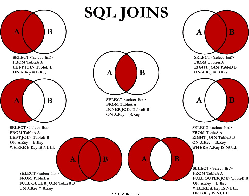